
Coordinating a massive amount of data in Microsoft Excel is a time-consuming headache. That headache can be made even worse when you need to compare data across multiple spreadsheets. The last thing you want to do is manually transfer cells using copy and paste. Thankfully, you don't have to. The VLOOKUP function can help you automate this task and save you tons of time.
I know, "VLOOKUP function" sounds like the geekiest, most complicated thing ever. But by the time you finish reading this article, you'll wonder how you ever survived in Excel without it.
Microsoft Excel's VLOOKUP function is easier to use than you think. What's more, it is incredibly powerful, and is definitely something you want to have in your arsenal of analytical weapons.What does VLOOKUP do, exactly? Here's the simple explanation: The VLOOKUP function searches for a specific value in your data, and once it identifies that value, it can find -- and display -- some other piece of information that's associated with that value.
How does VLOOKUP work?
VLOOKUP stands for "vertical lookup." In Excel, this means the act of looking up data vertically across a spreadsheet, using the spreadsheet's columns -- and a unique identifier within those columns -- as the basis of your search. When you look up your data, it must be listed vertically wherever that data is located.
The formula always searches to the right.
When conducting a VLOOKUP in Excel, you're essentially looking for new data in a different spreadsheet that is associated with old data in your current one. When VLOOKUP runs this search, it always looks for the new data to the right of your current data.
For instance, if one spreadsheet has a vertical list of names, and another spreadsheet has an unorganized list of those names and their email addresses, you can use VLOOKUP to retrieve those email addresses in the order you have them in your first spreadsheet. Those email addresses must be listed in the column to the right of the names in the second spreadsheet, or Excel won't be able to find them. (Go figure ... )
The formula needs a unique identifier to retrieve data.
The secret to how VLOOKUP works? Unique identifiers.
A unique identifier is a piece of information that both of your data sources share, and -- as its name implies -- it is unique (i.e. the identifier is only associated with one record in your database). Unique identifiers include product codes, stock-keeping units (SKUs), and customer contacts.
Alright, enough explanation: let's see another example of the VLOOKUP in action!
VLOOKUP Example
In the video below, we'll show an example in action, using the VLOOKUP function to match email addresses (from a second data source) to their corresponding data in a separate sheet.
Author's note: There are many different versions of Excel, so what you see in the video above might not always match up exactly with what you'll see in your version. That's why we encourage you to follow along with the written instructions below.
For your reference, here's what a VLOOKUP function looks like:
VLOOKUP(lookup_value , table_array , col_index_num , range_lookup)
In the steps below, we'll assign the right value to each of these components, using customer names as our unique identifier to find the MRR of each customer.
1. Identify a column of cells you'd like to fill with new data.
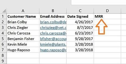
Remember, you're looking to retrieve data from another sheet and deposit it into this one. With that in mind, label a column next to the cells you want more information on with a proper title in the top cell, such as "MRR," for monthly recurring revenue. This new column is where the data you're fetching will go.
2. Select 'Function' (Fx) > VLOOKUP and insert this formula into your highlighted cell.

To the left of the text bar above your spreadsheet, you'll see a small function icon that looks like a script: Fx. Click on the first empty cell beneath your column title and then click this function icon. A box titled Formula Builder or Insert Function will appear to the right of your screen (depending on which version of Excel you have).
Search for and select "VLOOKUP" from the list of options included in the Formula Builder. Then, select OK or Insert Function to start building your VLOOKUP. The cell you currently have highlighted in your spreadsheet should now look like this: "=VLOOKUP()"
You can also enter this formula into a call manually by entering the bold text above exactly into your desired cell.
With the =VLOOKUP text entered into your first cell, it's time to fill the formula with four different criteria. These criteria will help Excel narrow down exactly where the data you want is located and what to look for.
3. Enter the lookup value for which you want to retrieve new data.

The first criteria is your lookup value -- this is the value of your spreadsheet that has data associated with it, which you want Excel to find and return for you. To enter it, click on the cell that carries a value you're trying to find a match for. In our example, shown above, it's in cell A2. You'll start migrating your new data into D2, since this cell represents the MRR of the customer name listed in A2.
Keep in mind your lookup value can be anything: text, numbers, website links, you name it. As long as the value you're looking up matches the value in the referring spreadsheet -- which we'll talk about that in the next step -- this function will return the data you want.
4. Enter the table array of the spreadsheet where your desired data is located.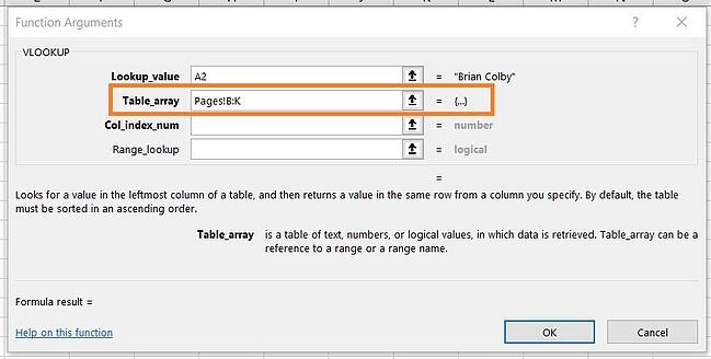
Next to the "table array" field, enter the range of cells you'd like to search and the sheet where these cells are located, using the format shown in the screenshot above. The entry above means the data we're looking for is in a spreadsheet titled "Pages" and can be found anywhere between column B and column K.
The sheet where your data is located must be within your current Excel file. This means your data can either be in a different table of cells somewhere in your current spreadsheet, or in a different spreadsheet linked at the bottom of your workbook, as shown below.
For example, if your data is located in "Sheet2" between cells C7 and L18, your table array entry will be "Sheet2!C7:L18."
5. Enter the column number of the data you want Excel to return.
Beneath the table array field, you'll enter the "column index number" of the table array you're searching through. For example, if you're focusing on columns B through K (notated "B:K" when entered in the "table array" field), but the specific values you want are in column K, you'll enter "10" in the "column index number" field, since column K is the 10th column from the left.

6. Enter your range lookup to find an exact or approximate match of your lookup value.

In situations like ours, which concerns monthly revenue, you want to find exact matches from the table you're searching through. To do this, enter "FALSE" in the "range lookup" field. This tells Excel you want to find only the exact revenue associated with each sales contact.
To answer your burning question: Yes, you can allow Excel to look for an approximate match instead of an exact match. To do so, simply enter TRUE instead of FALSE in the fourth field shown above.
When VLOOKUP is set for an approximate match, it's looking for data that most closely resembles your lookup value, rather than data that is identical to that value. If you're looking up data associated with a list of website links, for example, and some of your links have "https://" at the beginning, it might behoove you to find an approximate match just in case there are links that do not have this "https://" tag. This way, the rest of the link can match without this initial text tag causing your VLOOKUP formula to return an error if Excel can't find it.
7. Click 'Done' (or 'Enter') and fill your new column.
In order to officially bring in the values you want into your new column from Step 1, click "Done" (or "Enter," depending on your version of Excel) after filling the "range lookup" field. This will populate your first cell. You might take this opportunity to look in the other spreadsheet to make sure this was the correct value.
If so, populate the rest of the new column with each subsequent value by clicking the first filled cell, then clicking the tiny square that appears on the bottom-right corner of this cell. Done! All your values should appear.
VLOOKUP Not Working?
If you've followed the above steps and your VLOOKUP is still not working, it will either be an issue with your:
- Syntax (i.e. how you've structured the formula)
- Values (i.e. whether the data it's looking up is good and formatted correctly)
Troubleshooting VLOOKUP Syntax
Start with looking at the VLOOKUP formula that you have written in the designated cell.
- Is it referring to the right lookup value for its key identifier?
- Does it specify the correct table array range for the values it needs to retrieve
- Does it specify the correct sheet for the range?
- Is that sheet spelled correctly?
- Is it using the correct syntax to refer to the sheet? (e.g. Pages!B:K or 'Sheet 1'!B:K)
- Has the correct column number been specified? (e.g. A is 1, B is 2, and so on)
- Is True or False the correct route for how your sheet is set up?
Troubleshooting VLOOKUP Values
If the syntax is not the problem, how you may have an issue with the values you're trying to receive themselves. This often manifests as an #N/A error where the VLOOKUP cannot find a referenced value.
- Are the values formatted vertically and from right to left?
- Do the values match how you refer to them?
For example, if you're looking up URL data, each URL must be a row with its corresponding data to the left of it in the same row. If you have the URLs as column headers with the data moving vertically, the VLOOKUP will not work.
Keeping with this example, the URLs must match in format in both sheets. If you have one sheet including the "https://" in the value while the other sheet omits the "https://", the VLOOKUP will not be able to match the values.
VLOOKUPs as a Powerful Marketing Tool
Marketers have to analyze data from a variety of sources to get a complete picture of lead generation (and more). Microsoft Excel is the perfect tool to do this accurately and at scale, especially with the VLOOKUP function.
Editor's note: This post was originally published in March 2019 and has been updated for comprehensiveness.